From forecast to warehouse: judging demand predictions by what they cost
A team of five students connected demand forecasting to inventory and delivery decisions for an e-commerce marketplace. In a 13-week simulation, the best forecast cut cost 2.2–3.8% while filling 94% of demand.
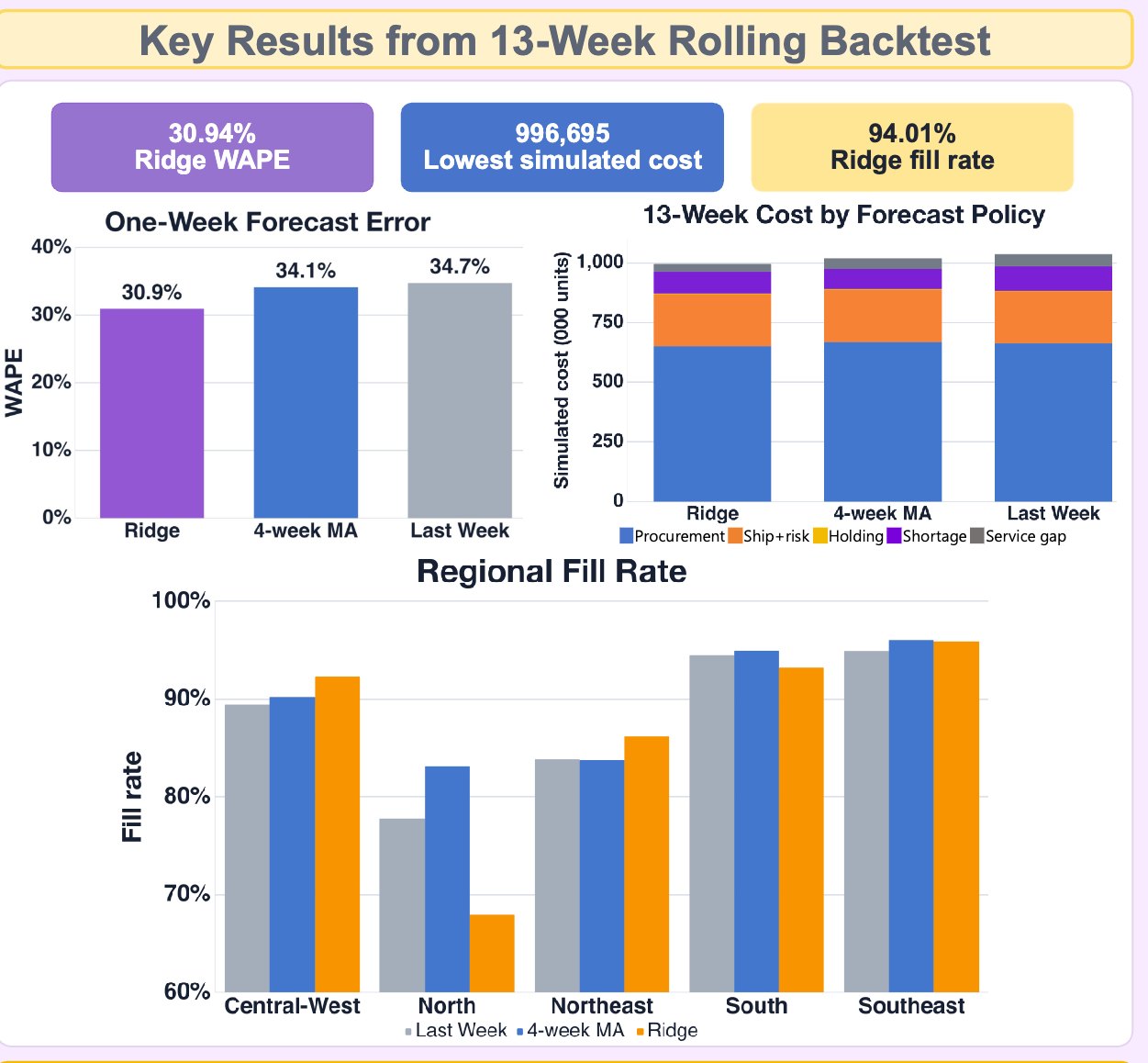
Inventory has to be placed before demand is known. Order too much and capital sits in warehouses; order too little and deliveries slip. Using 86 weeks of Brazilian e-commerce orders from Olist (112,634 order lines across 10 categories and 5 regions), this team compared three demand forecasts and fed each into a two-stage optimization: a four-week replenishment plan and a weekly fulfillment allocation across six candidate hubs. Over a 13-week rolling backtest, a Ridge regression forecast gave the lowest simulated total cost, 2.2–3.8% below the simpler baselines, at a 94.0% fill rate. The team argues forecasts should be judged by cost, inventory and service, not forecast error alone. Results are from simulation and do not represent Olist's actual operations.
Keywords · demand forecasting · inventory optimization · mixed-integer programming · fulfillment · e-commerce · rolling backtest
Who did this work
- Concentration focus
- AI + Business & Finance
- Concentration focus
- AI + Physical Intelligence
- Concentration focus
- AI + Business & Finance
- Concentration focus
- AI + Business & Finance
- Concentration focus
- AI + Physical Intelligence · AI + Business & Finance
Students are not named. Year of study is as of fall 2026. Direction and goal come from each student's own program plan.
1Stock has to be placed before demand shows up
An online marketplace decides weeks ahead how much of each category to hold in each regional hub. Overestimate demand and money is tied up in stock. Underestimate it and orders run out or ship late.
Forecasting and inventory planning are often handled separately, and forecasts are graded on error alone. The team asked whether a better forecast actually lowers operating cost once it drives real inventory and delivery decisions [1, 2].
2Forecast, plan, fulfill, repeat
- Prepared the data. 86 weeks of Olist orders [4], grouped into 50 demand series: 10 product categories across 5 regions.
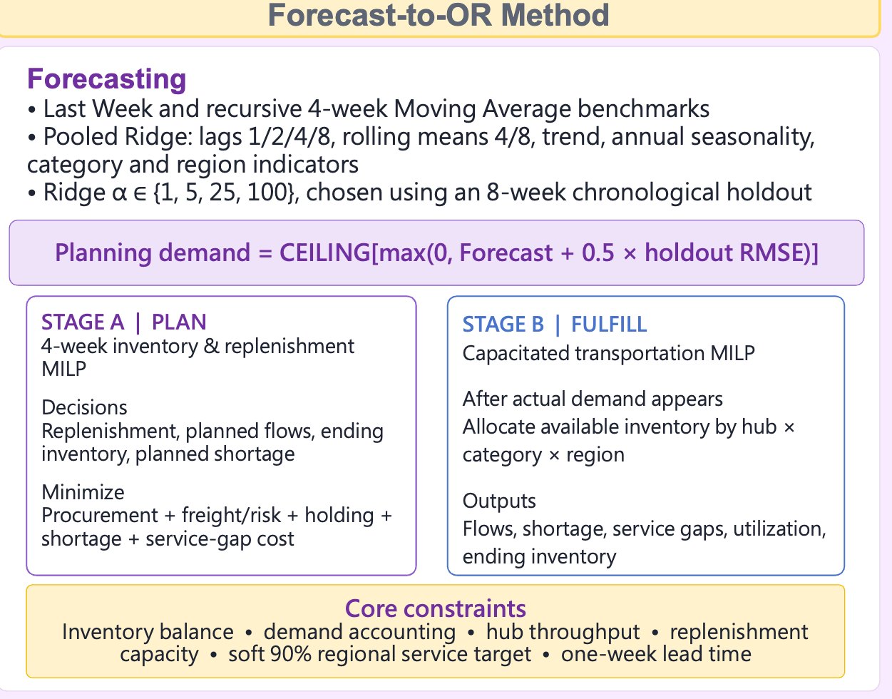
- Compared three forecasts. Last week's demand, a four-week moving average, and a pooled Ridge regression with lagged demand, trend, seasonality and category and region indicators [3].
- Added a safety buffer. Planning demand is the forecast plus half of the forecast's holdout error, so the plan accounts for how wrong the forecast tends to be.
- Planned stock (Stage A). A four-week replenishment model that minimizes procurement, shipping risk, holding, shortage and service-gap cost.
- Fulfilled orders (Stage B). Once actual demand appears, a capacity-limited model allocates stock from six hubs to regions, with a soft 90% regional service target.
- Rolled forward. Carried out only the first week of each plan, then re-forecast and re-optimized, for 13 weeks.
3The most accurate forecast was also the cheapest to run
| Scenario | Result |
|---|---|
| Ridge forecast, 13-week backtest | Lowest simulated total cost, 94.0% fill rate |
| Ridge vs. simpler forecasts | 2.2–3.8% lower simulated cost |
| No safety buffer | Fill rate drops to 86.0% |
| Full safety buffer (1x error) | Fill rate rises to 98.8% |
| Two-week lead time | Simulated cost rises about 9% |
| Hub capacity ±20% | No change; capacity was not the constraint |
4The poster
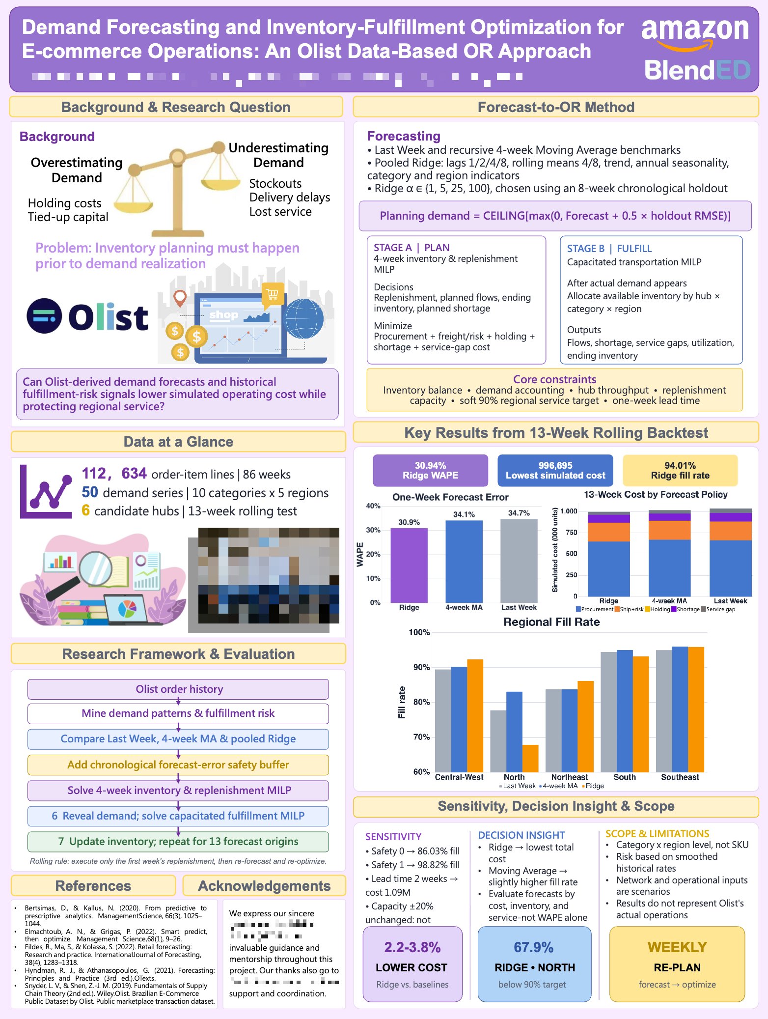
The team's poster from the On-Campus Experience. Student names and an event photo are blurred.
5What this does not show
- All costs and service levels come from simulation, not from a live operation.
- Network, cost and lead-time inputs are scenarios; the results do not represent Olist's actual operations.
- Demand is planned at category and region level, not for individual products.
- Delivery risk is based on smoothed historical rates.
6What this work shows the team can do
Researcher in Operations and Applied Machine Learning
Operations Management Researcher at MIT Sloan. Works on algorithmic equity and applied optimization. Studied Industrial and Systems Engineering at Georgia Tech.
The team built the forecasts and the optimization models and ran the backtest. The Project Lead worked with the team during the on-campus program and reviewed the models.
Operations research · Supply chain · Business analytics
An end-to-end model that ties a forecast to a cost a manager cares about reads well in both industry and graduate applications.
7What the Project Lead observed
After the project, the Project Lead wrote an evaluation of each student and placed each one on a four-level scale. This section shows the highest level reached on the team. The notes below describe the team's project. Individual ratings are not published.
System-Level Insight
- 1Foundational Application
- 2Applied Reasoning
- 3Independent Problem Solving
- 4System-Level Insight
Level 4 of 4: anticipates broader implications, risks or downstream effects, and connects technical decisions to real-world impact.
- Framing the problem
- Connected uncertain demand to inventory preparation and fulfillment performance, and tied the work to its business cost: overstock, shortages and delivery delays.
- Decisions and trade-offs
- Specified decision variables, objectives, constraints and assumptions, weighed procurement, inventory, transport, shortage and service costs, and checked how forecasts entered both optimization stages.
- Evidence and testing
- Used a simple last-week forecast as a benchmark and compared all forecasts by their downstream effect, not only by error.
- Limits and risk
- Separated the original Olist data from derived parameters and simulated assumptions, and checked whether simulated costs were reasonable before interpreting them for managers.
Where the Project Lead pushed further. Explain where the cost weights come from, define the error metric (WAPE) on first use, and interpret the key results rather than only report them.
Source: the Project Lead's written evaluations, August 2026.
References
- Bertsimas, D. & Kallus, N. (2020). From predictive to prescriptive analytics. Management Science, 66(3), 1025–1044.
- Elmachtoub, A. N. & Grigas, P. (2022). Smart "predict, then optimize." Management Science, 68(1), 9–26.
- Hyndman, R. J. & Athanasopoulos, G. (2021). Forecasting: Principles and Practice (3rd ed.). OTexts.
- Olist. Brazilian E-Commerce Public Dataset by Olist.
Join the AI in Operations Strategy – Amazon Project
This outcome came out of this project. Work with an operations researcher on a real supply-chain problem, and leave with something you can open and show.